Convex Hull Java Code

This page contains the source code for the Convex Hull function of the DotPlacer Applet. The code is probably not usable cut-and-paste, but should work with some modifications. I'll explain how the algorithm works below, and then what kind of modifications you'd need to do to get it working in your program.

How the convex hull algorithm works

1. First, it finds a point on the convex hull. In particular, it chooses the point with the lowest y coordinate. This is the code marked find highest particle below.
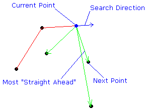
2. Then, it sets the direction of its search. Initially, this will be in the direction of the x axis.
3. Given a point and a search direction, it looks through all the points to find the point closest to "straight ahead". This point becomes the next point on the hull. The next search direction is the actual direction from the old point to the new one.
4. Step 3 is repeated as necessary.
   

   The running time for this algorithm is of order N times H, where N is the total number of points, and H is the number of points on the hull. For many arrangements of points, H is a lot smaller than N. On this page I give a table showing the expected number of points on the convex hull for various random arrangements of points. The table below shows information about the likely values of H for various values of N, for various distributions of points. Some explanation is in order.

   • For each value of N, I randomly selected N points according to some distribution. Then I calculated the number of points H on the convex hull.
   • In fact, I did this 1 million times for each value of N.
   • The table below shows
     • the average value of H,
     • the standard deviation
     • the skewness and excess kurtosis (calculated from these formulae
     for each distribution of points.
   • The four distributions of points are :
     • Uniform square : the N points are uniformly distributed in a square (side length 2).
     • Uniform circle : the N points are uniformly distributed in a circle (radius 1).
     • Uniform triangle : the N points are uniformly distributed in an equilateral triangle.
     • Gaussian : the N points are distributed on the plane according to a gaussian distribution.
   • This is more useful than it appears at first. The results for the square apply to any parallelogram, those for the circle to any ellipse, and those for the equilateral triangle to any triangle at all. Similarly, for the gaussian distribution, my covariance matrix is the identity, the same results should apply for any bivariate gaussian distribution of points.

   Anyway, as I said, you'll need to do some modifications to make the code below work, because of its idiosynchrasies. For example :

   • The code was in a class called ParticleSystem, which maintained an array a of Particle objects. Each Particle stored its position as an object pos of type Pt. This is almost certainly much more complicated than you need for your program.
   • The Pt class was just like java.awt.Point, except with a few useful vector manipulation methods added.
   • The method DLine just draws a line, bounding it within the drawing area.

   Enough explanation? Here's the code!

         public void DrawHull() {
         
         // draw the convex hull of the particles in the system
            if (a.length>1) {
               int i;
            // find highest particle
               double miny=a[0].pos.y;
               int mini = 0;
               for (i=1;i maxcos) {
                           nxti = i;
                           maxcos = thiscos;
                        }
                     }
                  }
                  DLine(a[curi].pos.x,a[curi].pos.y,a[nxti].pos.x,a[nxti].pos.y);
                  if (a[nxti].pos.diff(a[curi].pos).norm() != 0.0) {
                     dir = a[nxti].pos.diff(a[curi].pos);
                     dir = dir.scale(1/dir.norm());
                  }
                  curi = nxti;
               }
            }
         }
   

   This code is licensed under a creative commons license. Click the image below for more information.

   
   This work is licensed under a Creative Commons Attribution-ShareAlike 2.5 License.